This is my SuperMongo tutorial and help page. I will attempt to cover only the basic plotting commands of SM, but it should be enough to get you well on your merry SM way. SM is not hard to learn or use. However, it can be a little rough at first, simply because you have to learn quite a few commands before you can actually get anything done. Just be patient, and don't feel like you have to completely understand everything on this page the first time. A lot of it is optional (some of it I did not learn until years after I started), but you will want to use it eventually. Feel free to email with questions/comments/corrections.
I will certainly not cover everything SM is capable of. It can do
lots and lots of analysis and programming type things, but you will
have to find info on that elsewhere. I am just going to cover basic
plotting commands. For more info type help command or
apropos keyword in SM. Also, here are some great sites for
SM help (these are the sites that I learned SM from!):
The
Joy of Supermongo - The VERY BEST SM site there is.
Supermongo help - Brief but useful descriptions of a few common commands.
SM - Table
of Contents - This is the "official" SM page, but it is only
marginally useful. Most helpful is the listing of commands, which you
can also get by typing help in SM. The list
here is NOT complete by a long shot, but you will still find
interesting stuff. If you know where to
find a complete list of SM commands (and built-in macros), please let
me know.
SM only runs on Linux/Unix operating systems. Get it installed by your computer guru, open up a terminal and type sm. You can open SM in any directory you want. Whenever you open SM it will look for a file called '.smhist' in that directory. If it doesn't exist, it will make one. '.smhist' conatains your history of past commands. SM remembers what you did last time, and all of your setting from your last session are kept.
When you open SM, it will greet you, and you will be at the SM prompt. You can type commands individually into the SM prompt, but most often you will want to create a macro file which will contain a list of commands to be run consecutively.
The most important thing to remember when using SM is that once you change a setting, it stays that way until you change it again. That is, if you change the color to green, everything that comes after will be green until you change the color to something else. Sounds obvious, right? You'll be amazed to see how often you forget.
Miscellaneous Commands First, a word about case sensitivity. SM's commands are case sensitive in a weird way. A command must be in either all CAPS or all lower case (e.g. 'set' or 'SET' is fine, but not 'SeT'). Vectors and constants, however, are ALWAYS case sensitive (e.g. 'x' is different from 'X'). I just use all lower case because it's easy.help command: Gives you info on a command. Most of the commands I list here have more options available than I talk about.
apropos keyword: Finds topics in SM 'help' which are related to keyword.
!: Allows you to run shell commands from the SM prompt (e.g. !pwd).
#: Comment. The rest of the line is not read.
quit: This a very useful command indeed that lets you exit SM. I have often found that the exit command is something tutorials tend to forget, and when learning a new program, I am forced to just start trying every conceivable variant of 'quit', 'Quit', 'QUIT', 'exit', 'logout', etc. until I find the magic word that lets me the hell out.
SM data is held in vectors. This section explains the basics of vectors and the basic commands used to manipulate them.
Creating a Vectorset: This command can do an awful lot. Here are a few of the more useful implementations.
set vec={list}: Creates the vector vec. The individual elements of vec are referenced as vec[0], vec[1], vec[2], ... . The length of the vector is the number of elements.
set vec = min,max,delta: Create a vector starting at min, ending at max, with equal spacing delta. Extremely useful for plotting functions.
set vec = expr: Does arithmetic on vectors (i.e. performs the operation on all elements of the vector). If expr contains a vector, then vec will have the same length. If expr has multiple vectors, they must be of the same length. If expr has no vector, then vec will have length 1. You can do all the standard stuff, such as +, -, *, /, **, exp(), lg(), ln(), sin(), cos(), asin() acos(), sqrt(), and more. Try 'help expr' for a full list.
set vec = expr if(cond): This only performs the operation if cond (which contains at least one vector of the same length as any vector(s) in expr) is true. The length of vec will be less than or equal to the length of the vector(s) in cond. (See the example if you find this confusing.)
define const real: Does NOT deal with vectors, but defines a constant const to have the value of real. Once defined, a constant is referred to as $const.
print {vec1 vec2 ...}: Prints the vectors to the screen so you can take a look at them.
Examples:
set x=1,3,1 #equivalent to set x={1 2 3}
define c 2
set y=x+$c
set z=3*x+$c if(y<=4)
print {x y z}
Reading Data From a Filex y z 1 3 5 2 4 8 3 5
data "filename": Defines the datafile to read from. SM reads whitespace separated ASCII data files.
read {vec1 col1 vec2 col2 ...}: Reads in vectors of data from the datafile specified previously by 'data'. vec1,vec2,... are vector names; col1,col2,... are the columns in the dataset corresponding to those vecotrs. It won't read the data correctly if you have any strings (such as 'nan', 'inf', etc.) in your data.
Example:
data "./file.dat"
read {u 1 v 2 w 3}
If your 'file.dat' looks like:
then u={1e-2 5 9}, v={3 6.7 10}, w={4 8 1.1E2}.1e-2 3 4 5 6.7 8 9 10 1.1E2
Before you can make a plot, you have to set up your plot area, by choosing an output device, defining the size of the plot area, limits, the type of axes, etc.
Plot Area
device: Tells SM which device driver to output to. The most common are device x11 and device postencap "filename.ps" (or .eps if you prefer). x11 will output to a window on your monitor. For hardcopies, use postencap to create a postscript file. Remember that all plotting commands are written to the last device that was specified. Another quirk of SM is that the only way to close a device is to open a new one. Therefore, if you are writing to a postscript file, it will not be closed, and you will not be able to see the plot, until you open a new device. The easiest way to do this is to remember to close all postscript files with a device x11 or device nodevice command.
erase: Erases everything from the current output device. Useful for making sure your device is clear before you start plotting.
window nx ny x y: All arguments are integers. Divides up the page so you can put multiple plots on the same page. nx ny divide the page into nx equal columns and ny equal rows. x y specify which column and row you would like to plot in. For example, 'window 2 3 1 3' divides the page into 2 columns and 3 rows, and will plot in the first (left) column and third (top) row. The whole page is 'widnow 1 1 1 1'. If nx or ny is negative, then the axes are adjoining.
Axis Options
limits xmin xmax ymin ymax: Sets the limits for the plot. You can get SM to pick limits based on the data by 'limits x y' where you want to plot the vectors y vs. x.
ticksize smallx bigx smally bigy: Sets the spacing of the tickmarks. 'ticksize 0 0 0 0' tells SM to chose something appropriate based on the limits (I recomend sticking with this unless you know you want something special). Making smallx or smally negative makes that axis logarithmic (see 'Common Mistakes' for more info).
ctype: See 'Plotting the Data' below for description.
lweight: See 'Plotting the Data' below for description.
box: Draws the box around the plot area, icluding the tickmarks and labels. There are several options for changing the way box is drawn if you need to not have tickmarks or labels on an axis, or want to remove the axis entirely Try the SM help. If you need arbitrarily spaced tickmarks or string labels, you will have to look up the cumbersome axis command.
Now that we have data and we've set up the plot area, we can get around to the most important part of all, actually plotting the data.
Plotting Options
ctype color: Changes the color. Available colors are black, white, red, gren, blue, cyan, yellow, magenta. If you need more colors, try help ctype. The color actually afffects lots of stuff including the axes, the data points, and the labels.
ltype int: Changes the line style. int ranges from 0-6. 0 is a solid line, higher numbers have dots and dashes and whatnot. 'ltype' does NOT affect axes drawn by 'box', but does affect lines drawn by 'connect', 'draw', 'histogram', and 'errorbar', and even points drawn by 'points' and 'dot'.
lweight integer: Changes the width of lines. 1 is the default, and larger numbers give thicker lines. This option also will change the line width used for text, which is how you make text look bold. In general, the default lweight 1 is fine, but if you plan on shrinking the figure for publication, or intend to put it in a Powerpoint or other presentation, you should bump it up to lweight 2.
ptype int1 int2: Changes the point type for 'points' and 'dot'. int1 is the number of sides of the polygon the point is based on. int2 determines the style of the point (0=open, 1=vertices connected to center, 2=starred, 3=filled). Thus '3 3' is a filled triangle, '4 1' is an 'X', '6 2' is a 6-pointed star, and '10 0' is an open 10-gon, which looks just like a circle. '1 1' will give you very small dots. You can mix and match your polygons and styles as much as you like. Make sure you set 'ltype 0' before drawing points, or else they might look a little funny.
expand: See 'Labels' section below.
Plotting
connect xvec yvec: Draws lines connecting data points whose x coordinates are given by the vector xvec and y coordinates by yvec, which must be vectors of the same length. The points plotted will have coordinates (xvec[0],yvec[0]), (xvec[1],yvec[1]), (xvec[2],yvec[2]) ... .
points xvec yvec: Just like 'connect', except draws individual points instead of connecting them with lines.
histogram xvec yvec: Makes a histogram of height yvec at xvec.
error_x, error_y xvec yvec evec: Draws symmetrical error bars of length evec (evec must be a vector of the same length as xvec and yvec) in either the x or y direction around the points (xvec,yvec). If you want non-symmetric error bars, or error bars on a log scale, look up errorbar or logerr.
The final touch on our plots is labels.
Font Options
define TeX_strings 1: Defining the constant 'TeX_strings' (SM is case sensitive) to be '1' allows you to use TeX formating in your labels. Don't ask how it works, just be glad that it does.
expand real: Changes the size of points (drawn by 'points' and 'dot') and fonts drawn on the plot. 1 is the default, and it scales as the value you give it. i.e. 0.5 is half size and 2 is double size. One of SM's many whacky quirks is that if expand is exactly 1, then it can sometimes use odd fonts. It is always safest to never use exactly 1, but 1.001 or something similar instead.
ctype: See 'Plotting the Data' above for description.
lweight: See 'Plotting the Data' above for description.
Pre-Defined Positions
toplabel string: Puts a label at the top of the page. The label is always at the top of the page, and not at the top of a plotting area defined by a 'window' command. Kind of annoying, but easy to work around.
xlabel, ylabel string: Puts labels on the x and y axes. Can use TeX formating. These DO follow the plot area defined by 'window'.
User-Defined Positions
relocate x y: Sets the current location (used for labels, etc.) to (x,y). x and y are in the plot coordinates as defined by the axes. You can put set the current location to OUTSIDE the plot area if you want, by choosing (x,y) to be beyond the plot limits.
draw x y: Draws a line from the current location to the point (x,y). The current location is then set to (x,y). Uses the same options as 'connect' (ltype, ctype).
dot: Draws a point at the current location. Uses the same setting as 'points' (ptype, ctype, expand).
label string: Writes string at the current location. Uses the same options as other labels (expand, ctype).
I mentioned before that we could write a macro file which contains a list of commands to be run consecutively. You will want to do this almost all the time, because almost anything worth doing takes at least a dozen or two commands. To do this simply open your favorite text editor and create a file with a '.sm' extension. This is a macrofile.
The very first line of your macro should be your macroname. The macroname should NOT be indented, but all other lines MUST be indented. After that, you just put as many commands in the macro as you want (actually, I have had trouble reading macros that are over several hundred lines long). When you run the macro, these commands will just be run consecutively.
Before you can run the macro, you have to read it into SM. This is done by macro read macrofile. Once you have read the macrofile, you can run the macro by simply typing the macroname at the SM prompt.
To look at the postscript file you made, type !gv filename. If you need to change something (it will NEVER be perfect the first time), pressing the [up arrow] will cycle through your previous commands, just like in the terminal. Make the changes to your macro, read the new macro, run it, check it, repeat until everything is shiny and perfect.
Once you have the hang of that, a more advanced feature is that you can write multiple macros in the same macrofile. You can even run a macro by calling it from within another macro. To create multiple macros in a single macrofile simply begin every new macro with a non-indented line which is the macroname. A macro is just defined as the lines between the macroname and the start of the next macro, or the end of the file. Once a macro has been read (using macro read), it can be run just like any other command, by typing the macroname. You can have as many nested macros as you like. Some people prefer to have lots of little macros. I usually have just a few big macros, and only smaller macros when I need to do the same thing multiple times. There are lots of ways to do it, and this can be one of SM's most useful features.
Commands Out of Order
The most common mistake of all is one that I have referred to several times already. That is when you change a setting (such as device, limits, ctye, ltype, ptype, expand, etc.) it stays that way until you change it. Here are a couple of examples:
I hope you weren't expecting green points. They will be whatever color you last specified BEFORE you used 'points'. Even if the last time you changed the ctype was a month ago, it was stored in your '.smhist' file and SM remembers.points x y ctype green
Once again, 'points' is not going to write to the file "file.ps". It will use the device last specified BEFORE you used 'points'. I hope I am making my point abundantly clear. Don't feel bad when you forget, because you WILL forget. A lot. Even after you have been using SM for years. I just want you to be able to recognize and quickly fix such mistakes, because they usually are very simple to fix.points x y device postencap "file.ps"
Specifying a Setting Only Once
I also want to point out something that is NOT a mistake, and is actually good practice.
ctype black
     ...
box
     ...
points x y
connect x y
Logarithmic Axes
I mentioned before that using the command ticksize you can make logarithmic axes by making smallx or smally negative. However, it can be confusing because the limits and point coordinates are actually in log space. Here is an example of how to correctly make a log axis:
set x = {1 2 3 4 5}
set y = {0.1 1 10 100 1000}
set logy = lg(y)

limits 1 5 -1 3
ticksize 0 0 -1 10
box
points x logy
Here are some example macros that demonstrate most the of the commands I have gone over.
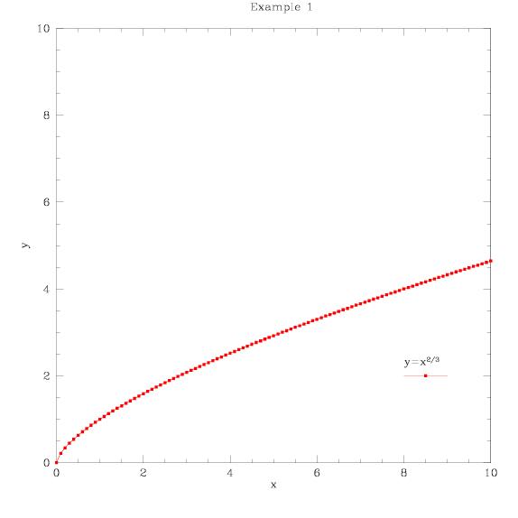
Example 1 shows a macro which makes a simple plot by using the commands listed above, in almost the exact order in which they are listed. It makes this plot.
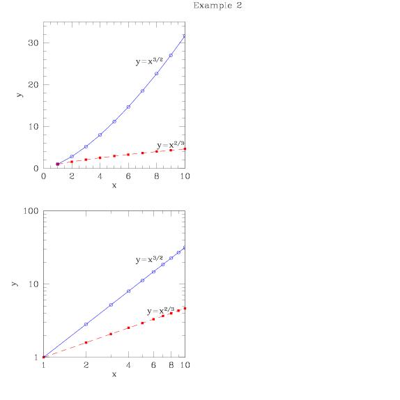
Example 2 makes this slightly more complex plot.
I hope all that was helpful and not terribly confusing, and I really hope none of it was just plain wrong.
Created by Craig Rudick, 2005.
Last modified 04/17/06.